Stochastic Differential Equations and Diffusion Models

Diffusion models (Sohl-Dickstein et al., 2015)(Ho et al., 2020) are one of the freshest flavors of generative models in the market right now (at least as of writing this post). They have been shown to outperform GANs in certain settings (Dhariwal & Nichol, 2021), and once trained, can also be used as feature extractors for supervised tasks (Baranchuk et al., 2021). As we shall see, they are also very elegant. The models are trained to invert a particular corruption process which corrupts a target distribution (say, the distribution of the images in your dataset) to approximately Gaussian noise. Once the inversion has been learnt, you can generate new samples from the target distribution by sampling Gaussian noise and passing it through the inversion process.

In particular, the diffusion models use a multi-step corruption process where, at each step, the input is scaled down (multiplied by a number less than one, not an image resize) and added with some zero-mean Gaussian noise. That is to say, the output of each step is a sample from a Gaussian distribution with its mean being a down-scaled version of the input. It is reasonable then, that the eventual distribution after many such steps would resemble a Gaussian. In this process, the scaling factor and the variance (or the covariance matrix in case of multi-dimensional data) are only a function of the step number.

The inversion process is defined in a manner similar to the corruption process, and goes from the last step to the first. The output of an inversion step is defined as a sample from a Gaussian distribution, but now, instead of the mean being a scaled version of the input and the variance being a (step number dependent) constant, they are defined using neural networks which take in the input and the step number and produce the two parameters.

Given this corruption and inversion model, variational inference can be used to learn the parameters of the neural networks involved. In particular, the corrupted variants obtained through the corruption process can be taken to be latent variables for which the posterior distribution is easily obtained. The corruption process then, can be taken to be the proposal distribution and an unbiased estimator for the evidence lower bound can be obtained (there are some algebraic tricks used, as in a variational autoencoder, to reduce the dependence on Monte Carlo estimates by using closed-form KL-divergences between Gaussians). More details can be found in this excellent blog posts: (Weng, 2021).

However, it is not immediately clear why these corruption and inversion processes are defined the way they are. Thankfully, an outstanding recent paper (Song et al., 2020) sheds a bit more light by relating the models to stochastic differential equations. In this blog post, we shall build up to the illustration in that paper from the ground up, armed with nothing but the Taylor approximation, the central limit theorem, our indomitable intuition and an abject disregard for rigour.

Discrete-Time Markov Processes

Let us start with getting a feel for Markov processes with discrete time and a discrete state space. Feel free to skip this section if you’re already familiar with them. Such a Markov Process is defined as a sequence of random variables $X_0, X_1, X_2, \dots$ with the property that given a particular random variable, the ones to its left are independent of the ones to its right. That is:

As a directed graphical model it looks like:

These random variables can be taken to represent the state of a system as it evolves stochastically through time, with the subscripts representing the timestamp. Thus, the Markov property, as defined above, seems a pretty natural one: it says that the future and the past are independent given the present. Based on this, the probability of an observed sequence $x_0, x_1, x_2, \dots$ can be neatly decomposed as:

Indeed, such a Markov process can be completely defined by the distribution of the initial state, $P(X_0 = x_0)$, and the transition probabilities $P(X_t = x_t | X_{t - 1} = x_{t - 1})$. Note how the latter is implicitly a function of $t$ because of the subscript. The transition probabilities from one state to another can be different for different times. We can also get the following intuitive recursion for the process fairly easily:

for $t \geq m \geq s.$ This follows from the fact that if we fix the state we encounter at time $m$ as $k,$ the probability of going from $x_s$ at time $s$ to $x_t$ at time $t$ is the product of the probability of getting to $k$ at time $m$ first and then continuing on to $x_t$ at time $t$ because of the independence assumption. Then, we can sum over all possible values of $k$ to marginalize it out (the derivation is fairly straightforward algebraically as well). In fact, in a similar manner we can also write an equation for the unconditional Marginal probability for $X_t.$ Note how this equation does not depend on the Markov property at all:

Finally, it is trivial to see that if $X_0, X_1, \dots, X_{T}$ is a Markov process, then so is its time-reversed version $X_T, X_{t - 1}, \dots, X_0$ since the past being independent of the future given the present is the same as the future being independent of the past given the present.

Continuous-Time Markov Processes

Now that we have seen markov processes where the time is indexed by discrete natural numbers, we can generalize it to the continuous case. To build our intuition, let us recall how we generalize discrete functions to continuous ones:

We increase the number of segments toward infinity by decreasing their width to nigh $0.$ However, intuitively, we also need to compensate for this infinite number of segments somehow to make sure the output of the function remains finite. We do so by decreasing the change in the function value for consecutive segments to almost zero as well.

We now want to divide the time axis of our Markov process in a manner similar to what we did with the x-axis. So how do we come up with such a compensation in the case of Markov processes? It turns out there are two ways to do so.

Jump Processes

The first way to maintain a sense of finiteness is by making the probability of state transition in an infinitesimal time segment $\mathrm{d}t$ infinitesimally small. This way, over a finite time period, there will be some finite probability of state transition. An example of this is the Poisson process which counts the number of random events in a given time. The process assumes that in an infinitesimal time segment $\mathrm{d}t,$ the probability of an event occurring is $\eta\mathrm{d}t$ with $\eta$ being the rate parameter of the associated Poisson distribution. We’ll not spend much time on the details since such processes are not our primary focus, but a wonderful reading for them is (Feller, 1949).

Diffusion Processes

Another possible continuous extension can be made in the case where the states of the system are real numbers (or vectors). In this case, we can formulate a sensible process if in an infinitesimally small time segment $\mathrm{d}t,$ the change in state is infinitesimal almost surely (recall that this change in state is stochastic). It is not immediately clear how to characterize such a transition function, but as we’ll see, it shows up quite naturally. In the next few sections we shall only consider a single-dimensional state space but the multi-dimensional case can be argued in a similar way with a bit more elbow grease.

The Kolmogorov Equations

To get a better sense of what the diffusion processes look like, we can start by writing similar equations for them as we did for the discrete case. Since now our state space is continuous, we will be dealing with probability densities instead of probabilities. Replacing the $\sum$ with a $\int$, the recursive equations from before become:

where the integral is understood to be over the entire state space. Here the notation has been simplified a bit such that $p(x;t|y;s)$ represents the probability density $p(X_t=x|X_s=y)$ with $t \geq s$ always. This notation more explicitly shows that this conditional density is a function of four variables $x, t, y$ and $s$.

As before, we have another equation that doesn’t depend on the Markov property:

We will use these equations to further probe the conditions required to come up with the “compensation” mentioned in the previous section. Before that, however, we can notice that the conditional probability density $p(x; t|y; s)$ and the initial marginal density $p(x; 0)$ should completely determine the entire diffusion process: given any collection of time points ${t_0, t_1, \dots, t_n}$, we can determine the joint density of the corresponding random variables (and hence characterize their distribution) using these two functions alone.

The Forward Kolmogorov Equation

Even if the evolution of the state-trajectory of a system in a diffusion process is difficult to grasp because of the infinities and the infinitesimals at play, we can perhaps try to describe the evolution of the conditional probability density function $p(x; t|y; s)$.

Let us consider the evolution of the conditional density function over a very small time interval $\mathrm dt$, and apply the recursive equation from earlier to it:

Here, the first multiplicand within the integral deals with a transition from $m$ to $x$ over a very small time period $\mathrm dt$. We know that over such a small time period, with a very large probability, the change in the the value of $X_t$ will be very small. It is difficult to characterize this “probably very small” change, but we can reparametrize the equation in terms of it. Let us call this change $\Delta$. In particular, let us define:

Note how this is a distribution over $\Delta$. We can visualize this reparametrization like so:

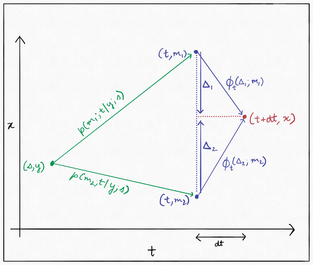
Based on this, we can rewrite the equation:

We can now Taylor expand the the entire function within the integral with respect to $m$ around $x$:

We can then use the fact that $\phi_t$ integrates to $1$ over $\Delta$, and that we can swap the order of integration and partial differentiation and get:

We now truncate the series to the second term, the justification for which will be presented in a bit. To get a sane limit on the right hand side, we must make sure that the first and the second moments of $\phi_t(;x)$ are of the order $\mathrm dt$. To that end, let us define:

Dividing by $\mathrm dt$ on both the sides we get the partial differential equation:

This is the Kolmogorov forward equation, also called the Fokker-Planck equation.

Let us now try to justify, retroactively, why we truncated the Taylor series up to the second moment. The fact is, that for “nice” distributions which are concentrated over an infinitesimally small region (which we assume $\phi_t$ is), you’d expect $\mathbb E[\Delta^3] \ll O(\mathbb E[\Delta]) = O(\mathrm dt)$ and $\mathbb E[\Delta^4] \ll O(\mathbb E[\Delta^2]) = O(\mathrm dt)$, and so we can ignore them (and higher moments). But then the question arises, why isn’t the second moment much smaller than the first one, and therefore negligible compared to $\mathrm dt$? It’s because the second moment is unsigned, so depending on how symmetric the distribution is, it is possible (though not necessary) that it matches or exceeds the size of the first moment. For example, a symmetric distribution would have a $0$ first moment, but can have an $O(\mathrm dt)$ sized second moment. Therefore, it makes sense for us to consider the largest odd and the largest even moment.

Deriving this PDE has automatically brought forward the “compensation” we talked about in terms of moments of $\phi_t$. In fact, $\phi_t$ actually serves as a distribution for the change in $X$ in time $\mathrm dt$. This allows us to talk about the small changes in $X$:

The function $f$ is called the drift coefficient of our diffusion process, and $g$ is called the diffusion coefficient. Based on this, we can separate out the location and the scale of the distribution of $\mathrm dX$ and write:

Where $\mathrm dw \sim D$ such that $D$ is some distribution with a variance of $\mathrm dt$ and a mean of $0$, and is independent of the current and past values of $X$. This equation is called the Ito diffusion SDE. I will now argue that we can always consider $D$ to be a Gaussian distribution, which will also tell us why the evolution of the probability distribution only seems to depend on the mean and the variance of the distribution but nothing else.

$\tiny{\text {someone please get this joke, i spent way too long on it}}$

Let us once again turn to the familiar land of deterministic functions. Suppose we are given a differential equation of the form

which we want to integrate to find $y(1)$ given the initial conditions $(0, y_0)$. How will we go about finding an approximate solution numerically? We can divide the interval $[0, 1]$ into $N$ pieces of width $\frac{1}{N}$ and assume that the value of $f$ is constant on each of these segments. Then, we can write the integral as:

where $f_i$ is the value of $f$ at the left edge of the $i\text{th}$ segment, and so, can be calculated as we go using the latest value of $y$. This is, in fact, Euler’s method for numerical integration. It makes sense then, that for a well-behaved $f$, as we make $N$ larger and larger and therefore the segment length smaller and smaller, we will approach the true solution.

We will now apply the same heuristic to our diffusion equation. Suppose we want to “integrate” our stochastic equation from $t=0$ to $t=1$ (really, the limits can be anything but $0$ to $1$ makes exposition easier). We divide our time from $0$ to $1$ into $N$ segments, and assume that the values of $f$ and $g$ are constant within a segment and equal to the values at the left edge. We can then write the integral as:

Notice how the $\mathrm dw$ has a hidden $\mathrm dt$ in it because it is a sample from a distribution with a zero mean and a variance of $\mathrm dt$. It is, however, not immediately clear how to simplify this “integral” any further.

Let us focus only on the integral in the second term, where we have the unwieldly $\mathrm dw$. The first thing to notice is that all the segments are independent since all $\mathrm dw$ are independent, so we can focus on only the first integral of $\mathrm dw$ from $0$ to $\frac{1}{N}$.

We can try discretizing this segment again into sub-segments and assume that in the $j\text{th}$ time sub-segment of length $\Delta t$, the change is a random variable $\Delta w_j$ with distribution $D$ with $0$ mean and $\Delta t$ variance. Then, intuitively, this “integral” can be represented as a sum, with the limit of $\Delta t$ tending to 0:

Now, by the Central Limit Theorem, the sum of those random variables should approach a Gaussian as we add more and more of them. The variance of this Gaussian would be the sum of the variances of all of them and should therefore be equal to $\frac{1}{N}$, while the mean will be $0$. So, we get that the integral on the left is a random variable such that:

Note that this is not an approximation, and we have resolved the limit here. (Also, the second parameter of the normal distribution will be the variance throughout this blog post.) This integral of $\mathrm dw$ is called the Brownian motion or the Wiener process.

We can now plug this back into our discrete approximation of the Ito equation and get (the $\Delta w$’s here are, of course, different from the ones introduced previously):

Here all of $\Delta w_i$ are independent Gaussian random variables with $0$ mean and $\frac{1}{N}$ variance. It makes sense, then, that as we increase $N$, this approximation will get tighter and tighter, and thus, $\mathrm dw$ can be treated as a $0$ mean Gaussian with variance $\mathrm dt \approx \frac{1}{N}$.

Let’s take a step back here. While arguing this, we have gone through two discretizations. Couldn’t we have gotten to the same point through just one? The fact is, we were able to convincingly resolve the first limit fully without any leftover approximations. This made arguing the second point much easier.

Finally, we can similarly argue about the unconditioned probability density evolution and get an unconditional forward equation (we just have to use the unconditioned recursive equation instead of the conditional one):

The Backward Kolmogorov Equation

The forward equation tells us how our conditional density evolves as the present time $t$ moves forward. However, what happens if we try to wiggle the time being conditioned upon? What happens if we condition on time $s - \mathrm ds$ instead of $s$? Indeed, the answer to that is an integral part of our recipe for reversing diffusion. The partial differential equation that that chronicles this wiggling is called the Kolmogorov “backward” equation. It describes the change in $p(x;t|y;s)$ with respect to $s$ (hence the term “backward”; recall that $t \geq s$). We can derive it in a manner very similar to the forward equation:

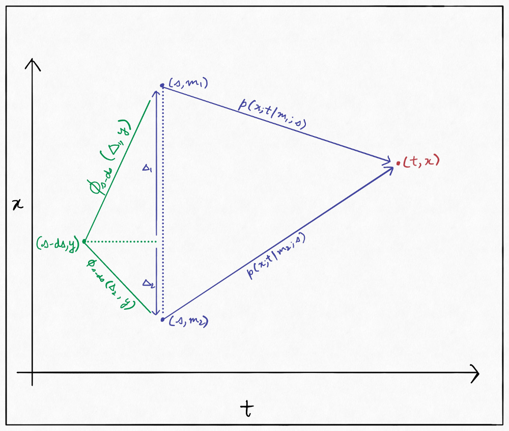
Based on this, we can write:

We truncate to the second moment for reasons described earlier and then apply the definitions from before. Taking the limit $\mathrm ds \rightarrow 0$ we get:

which is the Kolmogorov backward equation.

We now have two (three if you count the unconditional forward equation as separate from the conditional one) partial differential equations for the probability densities associated with our diffusion, which we will now use to describe the reverse of the diffusion process.

Reversing Time

We shall now look at a remarkable result from (Anderson, 1982) which tells us how we can describe the reversal of a diffusion process. But first, what do we actually mean by this reversal?

Suppose you have an initial distribution $p(x; 0)$ and some drift and diffusion coefficients $f$ and $g$. Together, they describe a distribution over the trajectories of your system through time. Suppose at time $T$, the marginal distribution of the state is $p(x; T)$. Can you describe a diffusion process such that it starts with a distribution $q(x; 0) := p(x; T)$ and evolves such that the distribution of the trajectories is the same as in the original process but with the time reversed? Of course, in such a case we shall have $q(x; T) = p(x; 0)$.

Going back to the example of the diffusion models mentioned in the introduction (forget that they have discrete timesteps for a moment), we start with the data distribution $p(x; 0)$ and follow a diffusion process such that $p(x; T)$ is a Gaussian distribution. The reverse-time diffusion in this case would be a process which starts with a Gaussian distribution and ends up with the data distribution, with the distribution of the trajectories being mirrored in the time axis.

Let’s once again try to harness some intuition from the deterministic case. Suppose we have:

Hmm, that seems rather easy. After all, we have:

Can’t we do something similar with our Ito SDE? It is also of the form:

Unfortunately, the deterministic variant doesn’t translate directly for us in this case. This is because in our SDE, the tiny Gaussian noise term $\mathrm dw$ is independent of the past values of $X$ but not of the future ones. So we can’t just slap a negative sign there and integrate from the future to the past by sampling $\mathrm dw$ independently of the values before it.

Thankfully, we can once again look at the flow of the probability densities. Since we know that the probability densities will remain the same in the reverse-time case except for the time-mirroring, all we need to do is get the Kolmogorov equations for $p(y;s|x;t)$ but with $s\leq t$. To do so, we can look at the joint density $p(x;t, y;s)$ and then try to convert it to the conditional form we desire. In particular, we will look at how it changes when we wiggle the $s$:

where in the last step we have just applied the backward and the unconditional forward equations. Dividing both the sides with $p(x;t)$, which is essentially a constant when considering only changes with respect to $y$ and $s$, we get:

The left hand side is all set, all we need to do is get the right hand side in the form of the forward Kolmogorov equation. In particular, we need to find drift and diffusion coefficients such that they are only a function of $x$ and $t$.

What follows is a rather filthy algebraic simplification and doesn’t seem to provide much insight. Feel free to skip it and go straight to the end, I just have it here for completion and also because (Anderson, 1982) skips the working (exercises for the reader amirite 🥲👍?). To make the notation cleaner, I will use $f_y$ to denote $\frac{\partial f}{\partial y}$ and $q$ and $p$ to denote $p(y;s|x;t)$ and $p(y;s)$ respectively. So it becomes:

We combine the first and the third term into the derivative of a product, and then add and subtract

\(\frac{\left(pg^2\right)_y}{2}\left(\frac{q}{p}\right)_y\) and combine these two new terms with the third and the fourth terms:

Finally, we add and subtract a copy of the third term, and combine a bunch of terms into product derivatives again:

Now, if we actually want to view the reverse process as a forward process with time index $u$, we should set $\mathrm ds = -\mathrm du$ so that $u$ ranges from $0$ to $T$ instead of $T$ to $0$. This change will help us compare with the form of the forward equation directly and extract the drift and the diffusion coefficients:

We can now immediately recognize the drift and the diffusion parameters from it and write the Ito SDE for the reverse case:

Following the convention in all the cited papers, we will instead write it in terms of $\mathrm dt = - \mathrm du$ (so that the time goes from $T$ to $0$ in the reverse case) and get:

The astute reader would’ve noticed the $\mathrm d\widetilde w$ here, instead of the regular $\mathrm dw$, because in that last step we have replaced the Brownian motion with a time reversed version such that $\mathrm dw$ has a variance of $-\mathrm dt$, since $\mathrm dt$ itself is negative. We can now get into the good stuff and see how this applies to diffusion models.

Diffusion Models as SDEs

Much of this section follows Appendix B of (Song et al., 2020), so it might be a good idea to huff it straight from the source now that we have all the tools to understand it. There are a few extra things explicitly derived here, so let’s keep moving forward.

First using good ol’ intuition, we generalize our results from the previous sections to the multidimensional case. However, we restrict the diffusion coefficient to be a scalar (or a scalar multiplied with the identity matrix) which only depends on the time $t$ and not $\mathbf X$. The forward SDE is:

Here $\mathbf f$ is a vector function and $\mathrm d\mathbf w$ is a sample from a spherical Gaussian with variance $\mathrm dt$ and with time ranging from $0$ to $T$. The reverse-time SDE is:

Here time ranges from $T$ to $0$ and thus $\mathrm dt$ is a negative increment, and $\mathrm d\mathbf w$ is a sample from a spherical Gaussian with variance $-\mathrm dt$.

Let’s put this aside for a bit and look at how diffusion models are defined. Given a data distribution $p_{D}(\mathbf x)$ that we wish to learn, the diffusion model is defined as a discrete process such that:

Here $\beta_t$ are some time dependent positive numbers less than $1$, and $\epsilon_t$ are standard spherical Gaussian noise terms independent of the past values of $\mathbf x$. The reverse process is then defined as:

Where $\mathbf \mu$ and $\mathbf \Sigma$ are neural networks which are trained such that the distribution of the forward trajectories matches the distribution of the reverse ones (see (Weng, 2021) for more details). $\gamma_t$ are standard spherical Gaussian noise terms independent of the future values of $\mathbf x$ (i.e. independent of $\mathbf x_u$ for $u > t$)

These discrete processes are reminiscent of our continuous time diffusion processes. We will now try to get a continuous approximation for the forward discrete process and see if it aligns with an SDE. We can then get a reverse continuous time process for it and try to match it with the reverse discrete process prescribed by the diffusion models.

Indeed, if the $\beta_t$ are small enough and the number of steps are large enough, we can replace $\beta_t$ with an infinitesimal function $\beta(t)\mathrm dt$ such that at each step, instead of moving $1$ unit forward in time, we move $\mathrm dt$ units. With this approximation, we have:

Using Taylor approximation to resolve the square root in the first term and recognizing that $\sqrt{\mathrm dt}\epsilon(t)$ is nothing but our good friend $\mathrm d\mathbf w$, we can write:

and therefore we can defined the reverse process as:

Discretizing this again, we see what exactly our $\mathbf \mu$ and $\mathbf \Sigma$ functions were trying to learn. In fact, we don’t even need to learn the $\Sigma$ function and we can just use the same coefficients as the forward process (Ho et al., 2020)!

One remaining piece of the puzzle that we haven’t looked into yet is why at the end of the forward process, at time $T$, the distribution can be considered a Gaussian with a mean of $0$ and a unit variance. We will now see that given a large enough $T$ and an appropriate $\beta$, we do eventually get there. To do so let us see what exactly is the form of the random variable at any arbitrary time $t$.

We will once again look to discretize the stochastic integral and evaluate devil-may-care limits, blowing all caution to the wind. Let’s start at time $0$ with $\mathbf x(0)$ and then go from there. The $\epsilon$’s, as before, are independent samples from the standard Gaussian (we have separated out the $\sqrt{\mathrm dt}$ standard deviation).

In the last expression, an invalid range (where the lower bound is greater than the upper bound) is understood to be just equal to 1 and 0 for products and sums respectively. This horrendous expression is surprisingly easy to deal with if we look at each of the terms individually and consider their natural logarithms.

Let’s start with the term with $\mathbf x(0)$. We get:

We assume that $n\Delta t = t$ and $\Delta t$ approaches $0$ so we can Taylor expand the logarithm. Truncating to the first term we get:

Taking the exponential to revert the logarithm we get:

The other term, which is a sum of products, is a bit more interesting. It is a sum of independent Gaussian samples, so the sum should be a Gaussian too. We just need to figure out its parameters. We know that the mean has to be zero since they individually have zero means, so we just need to find the variance. That is also rather easy. Since the noise terms are independent of each other, we can just take a limiting sum (or integral) of their variances (we are just working with variances instead of covariance matrices since everything is spherical).

The variance of a single noise term is simply:

We once again work in the log-space and get:

Further assuming that $i \Delta t = v$ and yet again Taylor abusing expanding the logarithm and converting the sum to an integral, we get:

Finally, to get the total variance, we can sum over $v$, which nicely turns into an integral:

We let everything inside the exponential be a variable and integrate by substitution and finally get:

Combining everything so far we get:

This form easily allows us to get samples from and conditional (on, say, $\mathrm x(0)$) statistics and density values for any arbitrary time-step. But the primary thing to notice here is that as the integral of $\beta(t)$ approaches infinity with time, the distribution of $\mathbf x(t)$ goes to a standard Gaussian which is what we wanted to show.

With this we have now seen that diffusion models are just discretizations of a particular SDE, and therefore have a corresponding reverse SDE as well. The reverse SDE then enlightened us about what exactly the neural networks in the diffusion models are trying to learn. Finally, we also justified the boundary condition of starting with a standard Gaussian distribution for the reverse diffusion process.

Score Matching

Once we know what exactly the neural network $\mu(; \theta)$ is trying to learn, we can use that to our advantage. We see that all we need to learn to formulate the reverse process is the term $\nabla_\mathbf x \log p(\mathbf x; t)$. Once we have this, we can fully characterize the reverse process given $\beta(t)$.

Let us only consider a particular time instant $t$ where we want to learn a parametrized function (say, a neural network) $s(\mathbf x, t; \theta)$ (with $\theta$ as the set of parameters) that predicts $\nabla_x \log p(\mathbf x; t)$. Intuitively, we can try to minimize the squared error:

This function (if we ignore all the $t$’s) is called the Fisher divergence between the learned distribution and the actual distribution. Minimizing this loss function is called “score matching” and is a well studied problem (Hyvärinen & Dayan, 2005). It is fairly easy to show that if two distributions agree on the gradient of the log-probability densities, they should be the same almost everywhere (line-integrate both the sides between two points and use the fact that probability densities integrate to $1$). Score matching may not always produce the same results as a maximum likelihood estimate, which minimizes the KL-divergence, but has some nicer stability properties when faced with noisy data (Lyu, 2012). It is also much more wieldy for high-dimensional distributions since we do not have to calculate the normalization constant for the density function since it is separated out because of the logarithm and then eradicated by the gradient operation.

As an aside, the score of a distribution is typically defined as the gradient of the log-density function with respect to a parameter and not the variable, which makes the “score matching” terminology particularly confusing. So, for example, the score of a Gaussian density $\mathcal N(x; \mu, 1)$ parametrized by $\mu$ will be defined as:

You can twist this definition a bit to achieve our definition by parametrizing the distribution with an additional “location” parameter $l$ such that: \(q(x; l) := p(x + l)\)

We can then calculate the score of $q$ at $l=0$ and reach our definition of “score”:

However, this arm-twisting doesn’t seem to yield any groundbreaking insights.

Going back to $\mathcal L_t(\theta)$, our dataset comprises samples from $p(\mathbf x; 0)$. We can easily get samples from $p(\mathbf x; t)$ by using the form of $\mathrm x(t)$ derived earlier, thereby getting a Monte Carlo estimate of the expectation. However, what we don’t have is the actual score function $\nabla_{\mathbf x_t}\log p(\mathbf x_t; t)$ to minimize the error against. Instead, we use the trick proposed in (Vincent, 2011) called “Denoising Score Matching.” The idea is to somehow rewrite this loss function so that we have a gradient of the conditional log-density $\log p(\mathbf x_t, t| \mathbf x_0, 0)$ instead of the marginal one. Based on the closed form from the last section, it is obvious that this conditional density will be a Gaussian with some pre-determined mean and variance, so computing it should be fairly straightforward.

The following is mostly a reproduction of the appendix of that paper in our context. We have:

Here the last term does not depend on $\theta$, so we can ignore it and only work with the first two terms. We will now use the following simple consequence of the chain rule:

If we only look at the second term in $\mathcal L_t$, we see:

Plugging this back into $\mathcal L_t$ and adding and subtracting $\mathbb E_{p(\mathbf x_0; 0)}\mathbb E_{p(\mathbf x_t; t)}\lVert \nabla_{\mathbf x_t}\log p(\mathbf x_t; t| \mathbf x_0; 0) \lVert^2$, which is independent of $\theta$, we get:

Of course, so far we have only focused on the Fischer divergence for a particular time instant $t$. Ideally, we would like to match it almost everywhere from $0$ to $T$. So we instead want to minimize:

We can rewrite this integral as an expectation over a uniform distribution, and also add a positive weighting function $\lambda(t)$ if we want to focus on certain time instants more than the others. This finally gets us to the loss function mentioned in (Song et al., 2020):

This loss is easy to get an estimator for. First we sample a time $t$ uniformly from $0$ to $T$. We then get a sample from our dataset, and then get a sample at time $t$ conditioned on our data point using the formula from the previous section. We can then calculate the weighted squared error between the gradient of this Gaussian log-conditional density and our model prediction. This gives us an unbiased estimator which we can optimize using some flavor of gradient descent.

Tl;dr

Diffusion models are discretizations of a continuous-time stochastic differential equation. Looking at the time-reversal of this diffusion process tells us that the neural network in the diffusion model is actually trying to learn the gradient of the probability density function with respect to the variable at different time instants. This itself is a well-studied problem called score matching.

Fin.

Citation

1
2
3
4
5
6
7

@online{dabral2021,
  author = {Dabral, Tanmaya Shekhar},
  title = {Stochastic Differential Equations and Diffusion Models},
  date = {2021-09-28},
  url = {https://www.vanillabug.com/posts/sde/},
  langid = {en}
}

Or:

1

Dabral, T. S. (2021, September 28). Stochastic Differential Equations and Diffusion Models. Retrieved from https://www.vanillabug.com/posts/sde/

References

1. Sohl-Dickstein, J., Weiss, E., Maheswaranathan, N., & Ganguli, S. (2015). Deep unsupervised learning using nonequilibrium thermodynamics. International Conference on Machine Learning, 2256–2265.
2. Ho, J., Jain, A., & Abbeel, P. (2020). Denoising diffusion probabilistic models. Advances in Neural Information Processing Systems, 33, 6840–6851.
3. Dhariwal, P., & Nichol, A. (2021). Diffusion models beat gans on image synthesis. Advances in Neural Information Processing Systems, 34.
4. Baranchuk, D., Rubachev, I., Voynov, A., Khrulkov, V., & Babenko, A. (2021). Label-Efficient Semantic Segmentation with Diffusion Models. ArXiv Preprint ArXiv:2112.03126.
5. Weng, L. (2021). What are diffusion models? Lilianweng.github.io/Lil-Log. https://lilianweng.github.io/lil-log/2021/07/11/diffusion-models.html
6. Song, Y., Sohl-Dickstein, J., Kingma, D. P., Kumar, A., Ermon, S., & Poole, B. (2020). Score-based generative modeling through stochastic differential equations. ArXiv Preprint ArXiv:2011.13456.
7. Feller, W. (1949). On the theory of stochastic processes, with particular reference to applications. Proceedings of the [First] Berkeley Symposium on Mathematical Statistics and Probability, 403–432.
8. Anderson, B. D. O. (1982). Reverse-time diffusion equation models. Stochastic Processes and Their Applications, 12(3), 313–326.
9. Hyvärinen, A., & Dayan, P. (2005). Estimation of non-normalized statistical models by score matching. Journal of Machine Learning Research, 6(4).
10. Lyu, S. (2012). Interpretation and generalization of score matching. ArXiv Preprint ArXiv:1205.2629.
11. Vincent, P. (2011). A connection between score matching and denoising autoencoders. Neural Computation, 23(7), 1661–1674.