The Kantorovich-Rubinstein Duality

In this post we’ll talk about the Wasserstein-1 distance, which is a metric on the space of probability distributions, and the Kantorovich-Rubinstein duality, which establishes an elegant and rather useful dual for it. One of the many good things about this metric is that in many cases it yields nicer gradients when compared to other divergences like the Jensen-Shannon divergence. For this reason, the Wasserstein-GAN (Arjovsky et al., 2017) trains the generator to minimize a loss that loosely mimics the W-1 distance between the model’s distribution and the target distribution. Calculating W-1 distance itself can be formulated as an optimization problem, and therefore it also admits a dual which, in fact, the critic in the W-GAN tries to approximately solve. As we shall see, the primal form is a pretty straightforward consequence of the definition, but the dual form requires some work to intuit.

This article presents the idea in the paper “On Translocation of Masses” by L. Kantorovich (Kantorovich, 1942) which is pretty neat, if a bit too terse. It also borrows a bit from C. Villani’s “Optimal Transport, Old and New” (Villani, 2008). The first couple of sections of this post introduce the idea behind the Wasserstein metric in its primal form, and then we formulate the dual problem from the primal without invoking any LP-duality magic to foster a better 𝓲𝓷𝓽𝓾𝓲𝓽𝓲𝓸𝓷™. Throughout the article we only look at discrete distributions and offer a silent yet heartfelt prayer to the gods of separability and hope it generalizes to distributions on $\mathbb{R}^n.$

The Wasserstein-1 Metric

In a land far, far away, the enigmatic Paradis Island has a set of cities $\mathcal{C}={c_1, c_2, c_3, …}.$ The distance between any two of these cities $c_i$ and $c_j$ is $d(c_i, c_j),$ where $d$ is a metric on $\mathcal{C}.$ That is, it’s a non-negative, symmetric function that’s zero iff $i=j$ and follows the triangle inequality. You know, all things that make distances distance-like. The cities cumulatively produce a single metric ton of potatoes, with each city $c$ producing $p(c)$ metric tons of the tasty taters. Unfortunately, the demand for the succulent spuds across the cities is not the same as $p.$ Instead, the demand in a city $c$ is given by $q(c).$ Thankfully, Paradis is self-sufficient and the total demand is the same as the total supply, i.e., one metric ton.

King Fritz has hired the Reeves transportation company to redistribute the tantalizing tubers to deal with this incongruity between the supply and the demand. The price they charge for transporting $m$ metric tons of the yummy yams from city $c_i$ to city $c_j$ is, understandably, $m\cdot d(c_i, c_j).$ The King hires us to come up with an optimal transportation plan that minimizes the burden on the royal treasury. This minimal cost is what’s called the Wasserstein-1 distance.

But what does a transportation plan look like? The transportation company requires instructions of the form “transport $m_{i,j}$ units from $c_i$ to $c_j$” for each ordered pair of cities $c_i, c_j.$ Additionally, all these instructions are carried out at the same time. So if a city $c$ originally had $m$ metric tons of the appetizing aloos (really scraping the bottom of the barrel here), it cannot send out more than $m$ units to other cities even if it has some potatoes incoming according to the plan. Of course, this restriction doesn’t change the minimal cost (why?). However, it does constrain the kind of instructions we can send over to our friends over at Reeves: the total mass going out of (or unmoved from) a city must be equal to the supply $p(c),$ and the total mass coming into (or unmoved from) a city must be equal to its demand $q(c).$

As you might have noticed, $p$ and $q$ represent probability distributions over $\mathcal{C}.$ Let $\gamma,$ a non-negative function over $\mathcal{C}\times\mathcal{C},$ be a valid transportation plan that we come up with such that $\gamma(c_i, c_j)$ tells us the amount of mass that must be transported from city $c_i$ to $c_j,$ with $\gamma(c, c)$ for any city $c$ representing how much of the mass is unmoved. Any valid plan must follow the following two equalities corresponding to the two constraints we formulated earlier:

The equalities also imply:

As mentioned before, another constraint is that of non-negativity. After all, you cannot transport negative mass:

All these together imply that any valid plan is, in fact, a distribution on $\mathcal{C} \times \mathcal{C}$ with its two marginal distributions being $p$ and $q.$ What then, is the total cost that we incur given a valid plan? It is, by definition:

where the subscript $d$ ties the cost to the specific metric over $\mathcal{C}$ being used. Let $\Gamma_{p, q}$ be the set of all valid plans following the constraints listed earlier. Then, we can define the Wasserstein-1 distance between $p$ and $q$ as the cost of the cheapest transportation plan that converts $p$ into $q$:

Indeed, this is the primal form of the Wasserstein distance.

Before we move any further, we should convince ourselves that $W$ is, in fact, a metric on the set of probability distributions on $\mathcal{C}$ and the introduction was not a lie. The non-negativity and the identity of indiscernibles (that is, $W_d(p, q) = 0 \iff p = q$) are easy to see given the fact that $d$ itself is a metric. It is also apparent that $W$ should be symmetric, since transforming $q$ to $p$ is equivalent to transforming $p$ to $q$ if we just reverse the arrow of time. Finally, the triangle inequality can be thought of as a consequence of the fact that $W$ is supposed to be the cost associated with the cheapest transportation plan. After all, if $W_d(p, q) \leq W_d(p, r) + W_d(r, q)$ did not hold for some distribution $r,$ we could always transform $p$ to $q$ by first transforming $p$ to $r$ and then transforming $r$ to $q$ and incur a smaller cost, contradicting our optimality condition for $W_d(p, q)$ (some hand-waving here, but it’s not that difficult to figure out).

The Optimal Plan

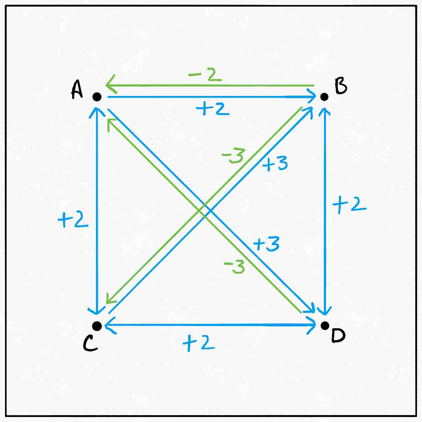
First of all, a trivial observation is that the optimal plan $\gamma^*$ may not be unique. Consider the example of points $A, B, C$ and $D$ forming a square:

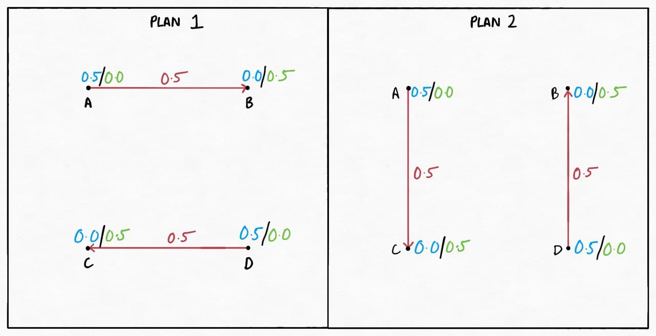
The edges represent the plan, with the numbers in red representing the amount of mass being transferred. The blue and the green numbers next to the nodes represent $p(c)$ and $q(c)$ respectively.

Both these plans can be easily verified to have the same (and optimal) cost. Clearly, it doesn’t matter how we match the deficits in $B$ and $C$ with the excesses in $A$ and $D$ since the distance covered is the same either way. Now the good ol’ King doesn’t really care about what plan we come up with as long as it’s optimal, so all we need to do is come up with one optimal plan.

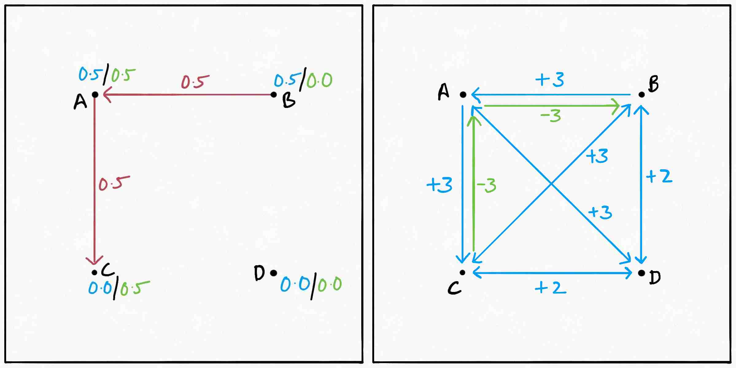
Inspired by how all the cool kids train their 9000-layered YOLONet-360, we decide to start off with an arbitrary but valid plan and take baby steps to improve it from there. So how do we go about doing that? Maybe the following sub-optimal plan will give us some ideas:

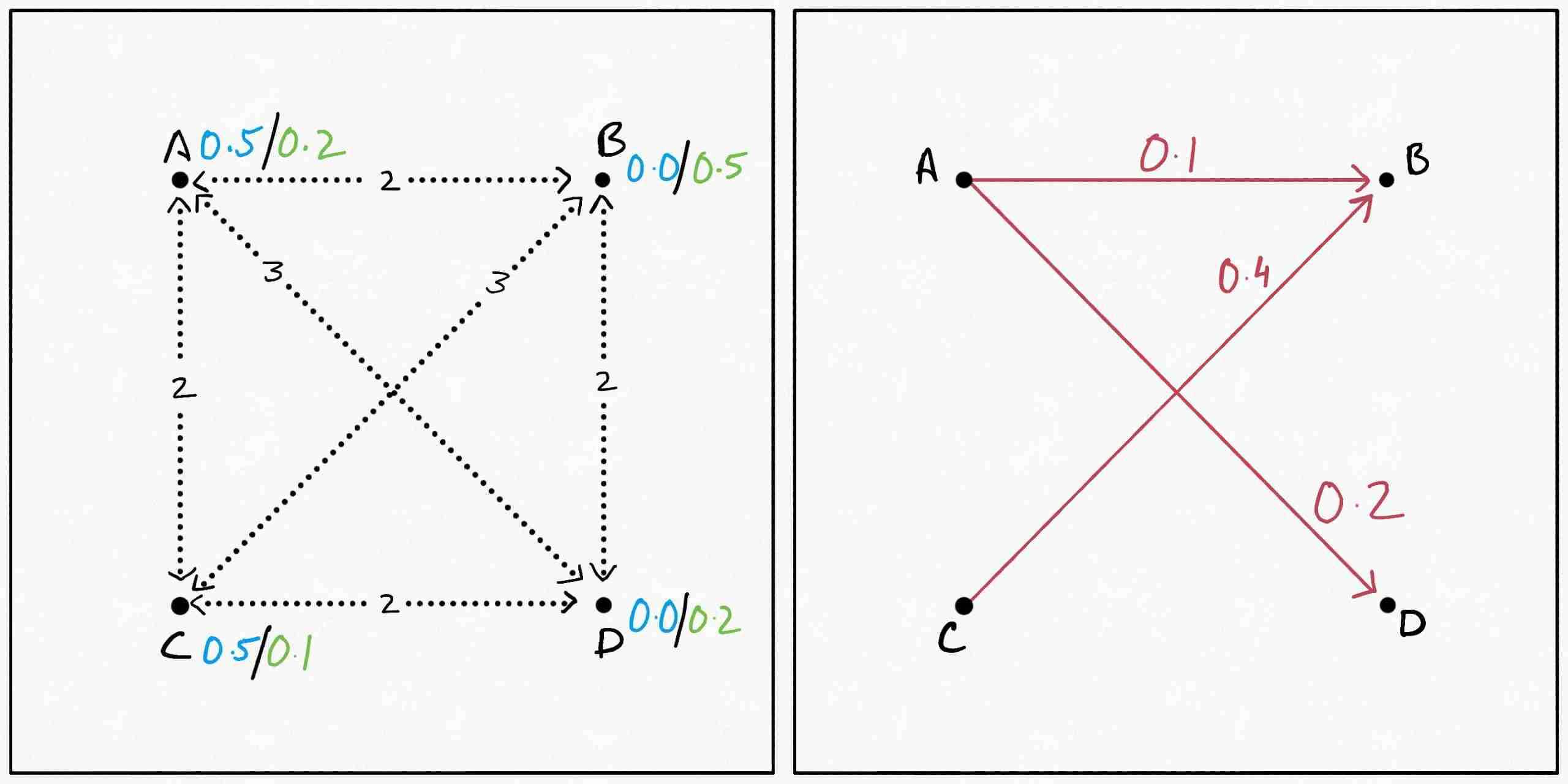
The first figure here with the dotted lines represents $d(x, y),$ since not all metric functions can be mapped to the 2D plane and I wanted to keep the distances rational. The second one represents the plan like in the previous example.

Suppose we decide that $D$ is too far from $A,$ so we want to try to reroute some mass $m$ out of the $0.2$ being transferred from $A$ to $D.$ If we subtract $m$ from $\gamma(A, D),$ $C(\gamma)$ changes by $-3m.$ But now $A$ has an excess of $m$ and $D$ has a deficit. To get rid of the excess in $A,$ let’s say we push it from $A$ to $B,$ costing us $2m.$ Now that $B$ gets this extra mass from $A,$ $C$ can decrease the $0.4$ units of mass it sends out to $B$ to $0.4-m,$ decreasing the total cost by $3m.$ Finally, $C$ can send over the excess $m$ to $D$ removing its deficit and adding $2m$ to the cost. In graphical form:

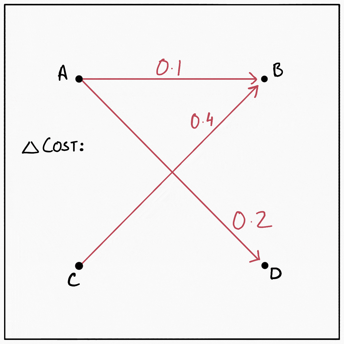
This cyclical sequence of operations retains the validity of the plan. After all, all we’ve done is reroute some mass $m$ from $D$ back to $D.$ The total change in the cost induced by it comes out to be $(-3 + 2 - 3 + 2)m = -2m.$ We would therefore like to reroute as much mass as possible through this cycle. So what is the maximum mass we can reroute? The first and the third operation in the cycle involve subtracting some mass from transfers present in the original plan. Since we cannot make $\gamma$ negative, the optimal value of $m$ becomes $\min \{\gamma(A, D), \gamma(C, B)\} = 0.2,$ and the new plan becomes:

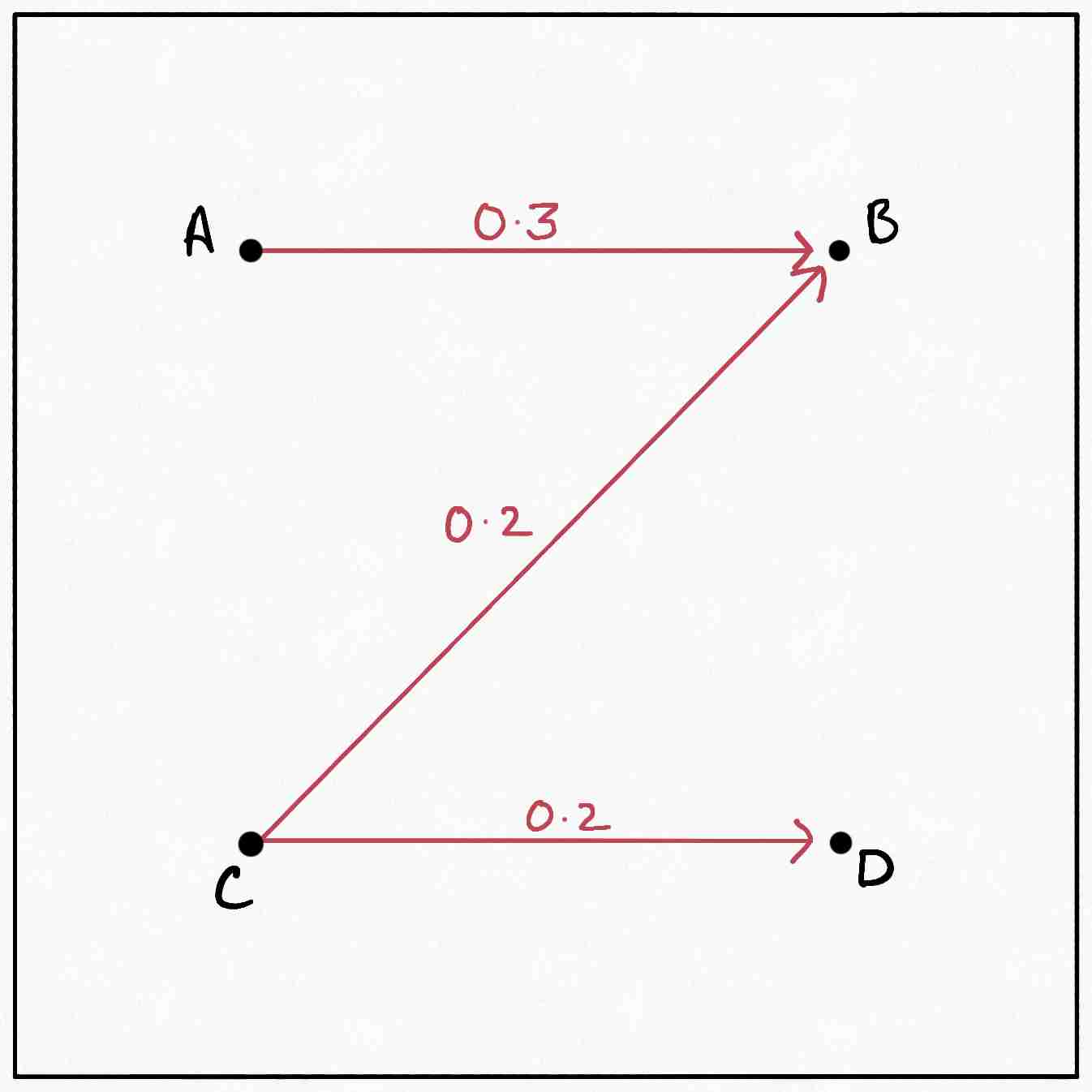
It’s easy to verify that the new plan is valid, and the cost of the new plan is $0.4$ less than the original plan.

In general, if from our original plan, we pick a list of $n$ non-zero transfers \(x_1\Longrightarrow x_2, x_3 \Longrightarrow x_4, \ldots, x_{2n - 1} \Longrightarrow x_{2n}\)

we can formulate a new, valid plan by rerouting some mass $m \leq \min \{\gamma(x_1, x_2), \ldots, \gamma(x_{2n-1}, x_{2n})\}$ through the cycle. In terms of the plan, this would result in $2n$ changes:

The idea is that for two consecutive transfers $x\Longrightarrow y$ and $a \Longrightarrow b$ in the list, we send $m$ units from $x$ to $b$ instead of $x$ to $y.$ We do so sequentially for all the members of the list, and finally we send $m$ units from $x_{2n-1}$ to $x_2$ instead of $x_{2n},$ completing the cycle and reestablishing the validity of the plan (it’s fairly easy to show algebraically that the new plan honors the validity constraints). The total change in cost would then be given by:

Now I know that the indexing is a bit wonky and the cyclic nature doesn’t pop out immediately. It’s better to write this as (recall that $d$ is symmetric):

Which nicely showcases the cycle that follows the propagation as \(x_2\rightarrow x_1\rightarrow x_4\rightarrow x_3\rightarrow x_6\rightarrow x_5 \ldots x_{2n} \rightarrow x_{2n-1} \rightarrow x_{2}\)

This cycle has a negative edge $x \rightarrow y$ if there is a transfer $y \Longrightarrow x$ and a positive edge otherwise. Notice the reversal in the order of $x$ and $y.$

Just to drive the point home, in our small example the list of non-zero transfers we considered was:

Notice that the non-zero transfer $A \Longrightarrow B$ was not necessary for our operation. We then changed the plan as:

The cycle in our case was $D \rightarrow A \rightarrow B \rightarrow C \rightarrow D,$ and the change in cost was:

As we did in our example, we would like to find a cycle which yields a negative total cost and then reroute the maximum possible mass $m = \min \{\gamma(x_1, x_2), \ldots, \gamma(x_{2n-1}, x_{2n})\}$ through it.

To do so, we can construct a complete graph which has negative edges from $x$ to $y$ with weight $-d(x, y)$ if $\gamma(y, x) > 0,$ and positive edges in all other cases with weight $d(x, y).$ We can then find negative cycles in such a graph and reroute some mass $m$ through them, decreasing the total cost. Notice how we haven’t picked a specific list of transfers here to form our negative edges, and have instead constructed the graph using all the available positive transfers. Indeed, a negative cycle in such a graph may have more than one consecutive negative edges. However, this won’t hurt us and using such cycles would still lead to a valid plan (why?). Borrowing some notation from max-flow/min-cut problems, let’s call this graph the residual graph of $\gamma.$

More concretely, the residual graph $G(\gamma)$ of a plan $\gamma$ can be defined as a complete, directed, weighted graph on $\mathcal C$:

The residual graph corresponding to the original plan is shown below. We can clearly see the negative cycle $D \rightarrow A \rightarrow B \rightarrow C \rightarrow D$ that we found earlier.

There is a subtlety here. In contrast to what was stated about more than one consecutive negative edges, if there are more than one consecutive positive edges in our negative cycle, applying it may not lead to a valid plan. The following figure illustrates one such example. The values for $d$ in the example are implicitly defined in the residual:

Consider the negative cycle $C \rightarrow A \rightarrow B \rightarrow D \rightarrow C.$ Unfortunately, since $D$ originally had $0$ mass, we cannot transfer any mass from $D$ to $C$ even though $D$ would be receiving the same amount of mass from $B.$

Clearly, the cycle strategy assumes that even if a node doesn’t have mass $m$ to spare, it can still send it out if it is receiving $m$ from another node, going against what we decided when formulating the problem. The negative edges don’t face this issue since they’re just returning some mass that was already being sent out in the original plan; the problem can only potentially occur when we have two (or more) consecutive positive edges in our cycle.

Thankfully, if we ever find such a cycle, we can always construct an equal or smaller (and therefore, still negative) cycle without the issue. Given a sequence of positive edges $s_0 \rightarrow s_1 \rightarrow s_2 \rightarrow \ldots \rightarrow s_n,$ we can replace it with the edge $s_0 \rightarrow s_n,$ which exists since our residual graph is complete. The weight of this edge can be $-d(s_0, s_n)$ or $d(s_0, s_n).$ If it’s the former, it’s obviously less than the sum of the original edges which were positive. If it’s the latter, it’s still less than the original by the repeated application of triangle inequality. In this example, we simply replace the two edge $B \rightarrow D \rightarrow C$ with a single, direct edge $B \rightarrow C,$ giving us the proper, applicable negative cycle $C \rightarrow A \rightarrow B \rightarrow C.$

This lengthy discussion has shown us that if we find a negative cycle in the residual graph, we can improve the plan using it. It may require some preprocessing before application as mentioned in the previous paragraph, but it will always improve the plan. Therefore, we know that the optimal plan must have no negative cycles in its residual. In other words, the absence of negative cycles in $G(\gamma)$ is a necessary condition for the optimality of $\gamma.$ But we can’t say, based on what we’ve seen so far, whether it is also sufficient. What if it was possible to reduce the cost incurred by a plan by radically changing it, even if there were no negative cycles? That is, what if we were in a “local minimum” of sorts? Spoiler alert: the condition is indeed sufficient, and the Kantorovich-Rubinstein dual in the next section will help us prove this.

The Kantorovich-Rubinstein Dual

It takes us three days and seventeen hours, but we eventually come up with a plan which has no negative cycles. We still don’t know whether such a plan is optimal or not, but at this point, we’re far too sleep deprived to do anything about it. Right as we are about to send over the potentially suboptimal plan to Reeves, we’re approached by Kenny the Ripper and his ragtag band of bandits with an offer to undercut the current contractors. To that end, they propose an alternative pricing scheme wherein instead of charging us in proportion to the distance traveled, they would charge us based on the starting and the ending point of a trip. Each city $c$ is assigned a particular “potential” $\phi(c)$ and transporting a mass $m$ from city $c_i$ to $c_j$ would cost $m \cdot(\phi(c_j) - \phi(c_i)).$ The total cost therefore becomes:

where the last step follows from the marginalization constraints on $\gamma.$ This shows us that $L$ does not depend on the plan $\gamma$ at all! We can therefore write it as $L_{p, q}(\phi),$ solely a function of the potential $\phi.$ The subscript ${p, q}$ ties the total cost calculated to the two distributions for the two expectation terms.

The catch is that they get to decide the values for $\phi.$ Being a part of a capitalist society, they would like to maximize the total cost incurred by us, and the optimization problem can now be looked at from their perspective. They, however, assure us that the differences in the values of $\phi$ would never exceed the distances among the cities:

Let’s call the set of potentials that honor this constraint given the metric $d$ as $\Phi_{d}.$ Notice how this constraint immediately implies that regardless of the choice of $\phi,$ $L_{p, q}$ for a given $\gamma$ would always be less than or equal to $C_{d}(\gamma)$:

This inequality doesn’t depend on the $\gamma$ in question as long as the plan and the potential are valid. Therefore, we can say:

The right hand side of the inequality is nothing but the primal form of $W_d(p, q),$ so it is always in our best interest to to take up Kenny’s offer. The left hand side, which Kenny needs to solve, is the Kantorovich-Rubinstein dual. The subscripts on the constraints and the cost functions explicitly showcase the duality. This inequality can be visually represented as:

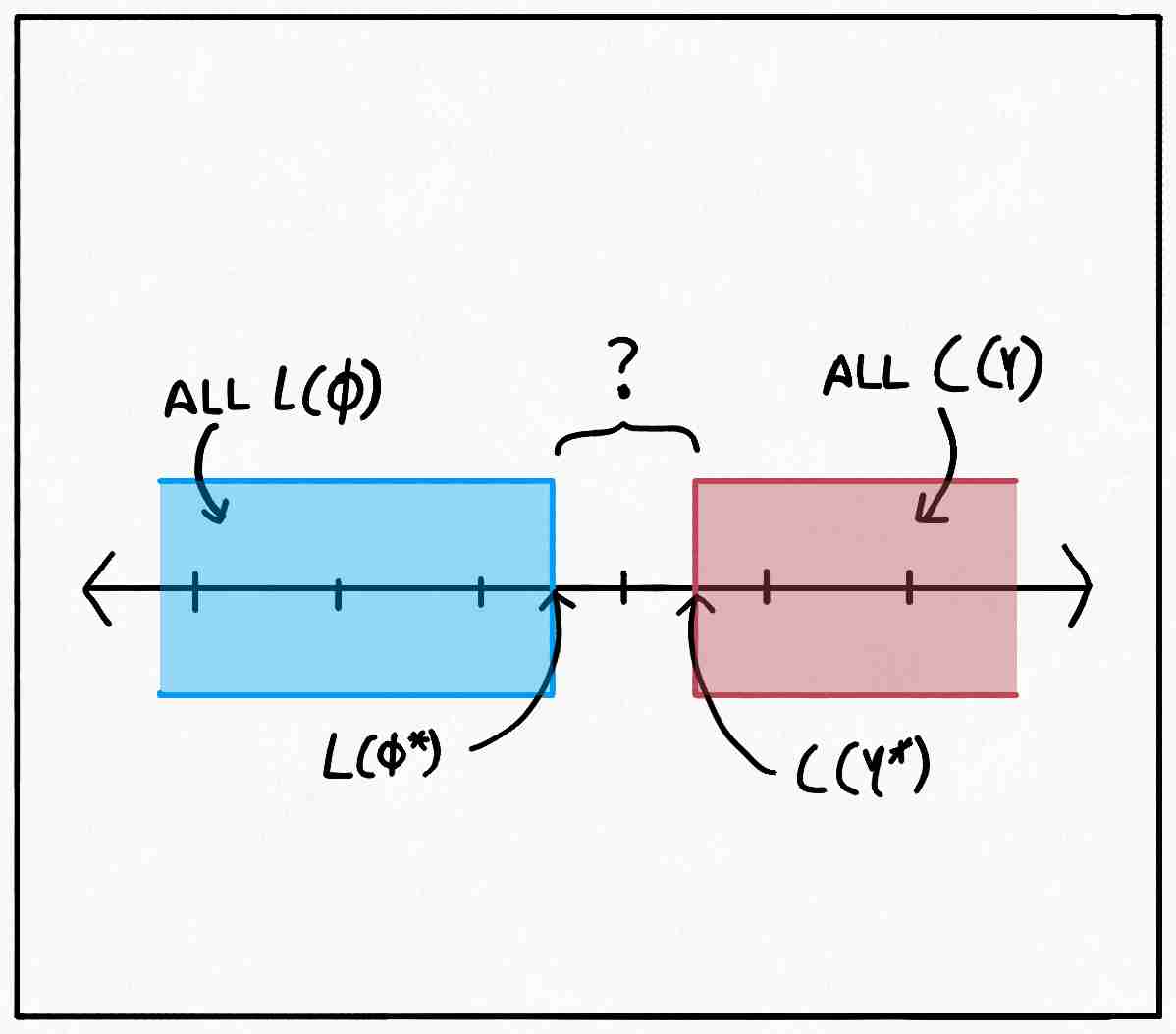
We don’t know if the gap between $L_{p, q}(\phi^*)$ and $C_d(\gamma^*)$ is zero or not. If only we could find any valid transportation plan and any valid potential function that produce the same value for the primal and the dual respectively, we would’ve shown:

• The found plan is optimal for the primal.
• The found potential function is optimal for the dual.
• The duality is strong so both the formulations are equivalent.

Indeed, we’ll start with a valid plan $\gamma’$ with the sole property that $G(\gamma’)$ has no negative cycles and construct an equivalent potential function, proving a fourth point:

• The absence of negative cycles in $G(\gamma)$ is both necessary and sufficient for the optimality of $\gamma.$

The thing to notice is that if we rearrange the constraints a bit:

it looks like something straight out of a shortest-path algorithm. In a directed, weighted graph, the length of the shortest path from a node $A$ to a node $B,$ let’s call it $l_A(B),$ must be less than or equal to the length of the shortest path from $A$ to another node $C$, $l_A(C),$ plus the weight of the edge from $C$ to $B.$ That is:

This is because if it weren’t, we could first go from $A$ to $C$ and then follow the edge from $C$ to $B$ and we will get a path from $A$ to $B$ shorter than the shortest path. Of course, in the case of $G(\gamma’),$ $w(c_i, c_j)$ may not be equal to $d(c_i, c_j)$ but we’ll come to that in a bit. Also, it seems awfully suspicious that the necessary condition for optimality that we found in the previous section was the absence of negative cycles, which is precisely the condition required to guarantee the existence of finite shortest paths. After all, if while looking for a shortest path between two nodes in a graph we were to encounter a negative cycle, we could traverse that cycle an arbitrary number of times and decrease the path length to $-\infty.$

Running with this hint, we define $\phi_{\gamma’}(c_i)$ to be the length of the shortest path between $c_0$ and $c_i$ in $G(\gamma’),$ where the choice of $c_0$ is arbitrary. As mentioned previously, this is a finite value for all $c_i$ since we are working with a complete graph with no negative cycles. By the Bellman-Ford equation from earlier, we see that:

where the second inequality comes from the fact that $w(c_j, c_i)$ can either be $d(c_i, c_j)$ or $-d(c_i, c_j).$ So, the $\phi_{\gamma’}$ described in this manner belongs to the valid set $\Phi_d.$ All that’s left is to show that $C_d(\gamma’) = L_{p, q}(\phi_{\gamma’}).$ If we take a look again at how we formulated the dual problem:

we can see that if $\phi(c_j) - \phi(c_i) = d(c_i, c_j)$ wherever $\gamma’(c_i, c_j) > 0,$ the sum would essentially boil down to:

We will now show that this is indeed the case by contradiction. First, we recall by the definition of $G(\gamma’)$ that $\gamma’(c_i, c_j) > 0$ implies $w(c_j, c_i) = -d(c_i, c_j).$ Now we assume the opposite of what we want to show: $\phi(c_j) - \phi(c_i) \neq d(c_i, c_j)$ for some $c_i, c_j$ where $\gamma’(c_i, c_j) > 0.$ Note that as we showed above, $\phi(c_j) - \phi(c_i)$ can’t be greater than $d(c_i, c_j),$ so under our assumption, it must be $< d(c_i, c_j).$ So our assumption is:

Let $c_x, c_y$ be one such pair that follows this condition. If we were to move from $c_0$ to $c_y$ along the shortest route, and then move to $c_x$ along the edge $c_y \rightarrow c_x,$ which has a weight of $-d(c_x, c_y),$ the total length of the path would be $\phi_{\gamma’}(c_y) - d(c_x, c_y)$ which is then less than $\phi_{\gamma’}(c_x)$ by our assumption. But this raises a contradiction to the definition of $\phi_{\gamma’}(c_i)$ as the length of the shortest path from $c_0$ to $c_i,$ so our assumption must be flawed. That is, $\gamma’(c_i, c_j) > 0$ must imply $\phi(c_j) - \phi(c_i) = d(c_i, c_j).$ This, in turn, proves the equality:

for any $\gamma’ \in \Gamma_{p, q}$ such that $G(\gamma’)$ has no negative cycles. This result itself then proves the list of things that were mentioned above, including the much coveted result:

And this concludes our little adventure.

P.S. This discussion doesn’t show whether the algorithm of repeatedly eliminating negative cycles terminates or not. That’s a story for some other time (or maybe not). For today, I think we’ve had enough of potentials and plans.

Citation

1
2
3
4
5
6
7

@online{dabral2020,
  author = {Dabral, Tanmaya Shekhar},
  title = {The Kantorovich-Rubinstein Duality},
  date = {2020-08-28},
  url = {https://www.vanillabug.com/posts/wasserstein/},
  langid = {en}
}

Or:

1

Dabral, T. S. (2020, August 28). The Kantorovich-Rubinstein Duality. Retrieved from https://www.vanillabug.com/posts/wasserstein/

References

1. Arjovsky, M., Chintala, S., & Bottou, L. (2017). Wasserstein gan. ArXiv Preprint ArXiv:1701.07875.
2. Kantorovich, L. V. (1942). On the translocation of masses. Dokl. Akad. Nauk. USSR (NS), 37, 199–201.
3. Villani, C. (2008). Optimal transport: old and new (Vol. 338). Springer Science & Business Media.